6 Density-independent Population Growth: Humans on the rise

Figure 6.1: Earth has now entered the Anthropocene. Geologists are debating precisely when that happened.

Reproduction helps define what we call “life”, and leads to exponential growth. This chapter introduces this concept and how we quantify it.

6.1 Goals

In this chapter, you will

learn the two fundamental principles of population growth,
do a little math: practice calculating rates of population growth,
do a little programming: use a “for-loop” to do lots of work very easily,
determine how the rate of human population growth has changed over time, and
start to develop a greater understanding and intuition for exponential rates.

In this chapter, we’ll use these techniques and data from Our World in Data to describe mathematically the growth rate of the world’s human population at different points in time over the last 10,000 years.

6.2 Preparatory Steps

Watch these videos: lectures 3a and 3b before proceeding.

Go to our class data repository, and download HumanPopData-2023-0101.csv. Make sure the file remains in the same simple format, “comma separated values” (.csv).

If you are curious, check Deliverables, at the end.

6.3 Background

Given sufficient resources, life is autocatalytic – the products of reproduction (offspring) amplify the rate of reproduction, leading to exponential growth.

As ecologists, we can state this with the following propositions (Hastings 2011):

A population grows exponentially in the absence of other forces.
There are forces that can prevent a population from growing exponentially.

This deceptively simple pair of propositions provides a basis for an enormous amount of ecology. They are analogous to Newton’s First Law of Motion:

Every body perseveres in its state of being at rest or of moving uniformly straight forward, except insofar as it is compelled to change its state by forces impressed. (The Principia: Mathematical Principles of Natural Philosophy (1687), 3rd edition (1726), trans. I. Bernard Cohen and Anne Whitman (1999), Axioms, or Laws of Motion, Law 1, 416.)

Now we would say that a body remains at rest, or in motion at a constant speed in a straight line, unless acted upon by a force.

The first proposition of population growth can emerge as the consequence of the following assumptions:

all individuals in a population are identical.
there is no migration in or out of the population.
1. the number of offspring per individual (or the per capita birth and death rates) are constant through time, and (ii) independent of the number of individuals in the population.

Deviations from these assumptions lead to proposition 2, and most of the interesting parts of single species population dynamics (Hastings 2011).

However, although propositions 1 and 2 can follow from assumptions a-c, these assumptions are not necessary. For instance, in some cases, individuals don’t need to be identical, and we deal with a big exception in the next chapter where we introduce structured population growth. Also, migration is admissible, provided immigration = emigration and that it doesn’t alter the rate of change. Nonetheless, other deviations from a and b can have very important consequences for single species population dynamics. We will get to those in later chapters.

Even when populations don’t grow exponentially, we often describe population growth using the same mathematical approach. We do that for at least a few of reasons:

approximations of more complicated dynamics often simplify to exponential growth under reasonable assumptions,
over short periods of time, deviations to exponential growth still result in patterns that are very similar to exponential growth, and
we typically don’t know precisely what mechanisms limit exponential growth or by how much, and therefore exponential growth is as good a mathematical description as any.

If you have not already done so, watch lectures 3a and 3b before proceeding.

6.3.1 Population growth of Homo sapiens: a case study

The human population shares many features with other populations. Like other species, humans are distributed unequally around our available habitats, we consume resources and produce waste products, and the size of our population changes over time.

Humans, as we would we recognize ourselves, have been around for ~300,000 years. Since that time a lot has happened to us, and we have done a lot to alter the planet. About 10,000 years ago, we started to use agriculture to raise a lot of our food, in the agricultural revolution. Oddly, this seems to have contributed simultaneously to both a decline in life span due to poor health, and yet also an increase in population growth rate and a corresponding increase in population size. The state of the human population is dynamic and undergoing transitions that are in different stages in different places around the world (Lee 2011).

Here we examine changes in human population size from 10,000 y ago to 2021. The data are estimates, and we have annual estimates with increasing greater frequency, up until 2021.

We will calculate the density-independent per capita growth rate for pairs of years in the data set. We’ll do this by written out by hand, and also in R, using code to do everything quickly, efficiently and, importantly, reproducibly, so that you–or anyone–could check your estimatation procedure.

Recall from lecture (link above) that we often use estimates of \(\lambda\) and \(r\) to quantify how rapidly a population is growing (or declining) at various points in time. For a population with overlapping generations and reproducing continuously, we can estimate the per capita exponential growth rate at a particular point in time (\(r_t\)) using the following equation:

\[r_t = \frac{\frac{\ln N_{t+h}}{\ln N_t}}{(t+h) - t} \tag{6.1}\]

where \(N_t\) is the size of the population at some starting time point \(t\), and \(N_{t+h}\) is the size of the population after some time interval \(h\), and \(\ln\) is the natural logarithm.

For example, imagine we that in 2020, we had 100 mice and exactly two years later, the population had grown to 150 mice. Here are the values that we would use to calculate \(r_t\):

\(t = 2020\)
\(t+h = 2022\)
\(h = (t+h) - t = 2022-2020 = 2\)
\(N_t = 100\)
\(N_{t+h} = 150\)

We would substitute these values into the above formula (#eq-r) as,

\[\begin{align*} r_t &= \frac{ \ln \frac{150}{100}}{2022 - 2020}\\ &=\frac{\ln 1.5}{2}\\ &= 0.2027 \end{align*}\]

showing each step of our work. Whenever you need to show how you arrived at an answer (such as in homework, research, or in a job), you should do something like this.

When \(r_t\) is positive (\(r_t > 0\)), this means that the population was growing, and quantifies how fast it grew and became larger.

What if we reverse so the we started with \(N_t = 150\) and the population declined to \(N_{t+h} = 100\)?

\[\begin{align*} r_t &= \frac{\ln \frac{100}{150}}{2021 - 2020}\\ &=\frac{\ln \frac{2}{3}}{2}\\ &= -0.2027 \end{align*}\]

ending with a negative value (\(r_t < 0\)), indicating that the population shrank. When \(r_t < 0\), that means the population has decreased in size. Sometimes we call that “negative growth”.

What do you think we we get if the population didn’t change, so that \(N_t = N_{t+h} = 100\)?

6.3.2 Projecting population size into the future

If we make certain assumptions, we can make predictions about the future. In order to make predictions about the size of the population next year, or in 5, 10, or 20 years, we can extrapolate the current rate of change into the future. To do that, we can use the instantaneous rate of increase, \(r\), and the amount of time, and a solution from calculus.

To predict the size of a population to year \(t\) from some starting time, we rely on the rule that,

\[N_t = N_0 e^{rt} \tag{6.2}\]

or equivalently,

\[N_{t+h} = N_t e^{rh}\]

where the parameter \(r\) is the per capita instantaneous rate of increase, and \(t\) is the amount of time, or time interval. The letter \(e\) is the exponential, or Euler’s constant. The exponential is the base of the natural logarithm. The important thing here is the time interval in the exponent (\(t\) or \(h\)) has to be the time interval from the starting value of \(N\) to the projected value of \(N\).

Figure 6.2: Common duckweed (*Lemna minor*) populations can grow fast. Credit: https://commons.wikimedia.org/w/index.php?curid=1085476

Imagine we have a population of the small floating plant duckweed (Lemna minor), that can double in about two weeks . In that case, \(r = 0.35\) new lemna per old lemna per week. Pretend we start with a population of 100 lemna individuals (\(N_0 = 100\)). How many lemna should we have in three weeks? Show your work (e.g., Figure 6.3).

Figure 6.3: Projecting the size of the duckweed population three weeks into the future.

(Overthinking: Equation 6.2 is derived from the growth equation Equation 6.1 using integral calculus. It is the integral from 0 to t of Equation 6.1.)

6.4 Methods

Make sure your working directory is Rwork.
Load the necessary packages.

library(tidyverse) # for readr, dplyr and others

── Attaching core tidyverse packages ──────────────────────── tidyverse 2.0.0 ──
✔ dplyr     1.1.4     ✔ readr     2.1.5
✔ forcats   1.0.0     ✔ stringr   1.5.1
✔ ggplot2   3.4.4     ✔ tibble    3.2.1
✔ lubridate 1.9.3     ✔ tidyr     1.3.1
✔ purrr     1.0.2     
── Conflicts ────────────────────────────────────────── tidyverse_conflicts() ──
✖ dplyr::filter() masks stats::filter()
✖ dplyr::lag()    masks stats::lag()
ℹ Use the conflicted package (<http://conflicted.r-lib.org/>) to force all conflicts to become errors

library(patchwork) # to combine ggplot2 figures

6.4.1 Load data

Next, we get the data, if you haven’t already done so.

Go to our class data repository, and download HumanPopData-2023-01-01.csv. Make sure the file remains in the same simple format, “comma separated values” (.csv).
Put HumanPopData-2023-01-01.csv in your working directory, Rwork.
Open HumanPopData-2023-01-01.csv and make note of the first three lines of metadata. When you close the file, do not save any changes, and make sure not to save it in a new format, such as “.xlsx” or “.numbers”.
Continue to make sure the file remains in the same simple format, “comma separated values” (.csv).

Now import the data into R, and glimpse the structure of the data frame.

d <- read_csv("HumanPopData-2023-01-01.csv", 
              skip=3 # skip three lines of metadata
              )

Rows: 259 Columns: 2
── Column specification ────────────────────────────────────────────────────────
Delimiter: ","
dbl (2): Year, est.N

ℹ Use `spec()` to retrieve the full column specification for this data.
ℹ Specify the column types or set `show_col_types = FALSE` to quiet this message.

glimpse(d)

Rows: 259
Columns: 2
$ Year  <dbl> -10000, -9000, -8000, -7000, -6000, -5000, -4000, -3000, -2000, …
$ est.N <dbl> 4432266, 5616996, 7242892, 9577918, 13201832, 19075771, 28774661…

Note that years before the current era (BCE) are negative numbers, while numbers in the current era (CE) are positive.

Let’s also graph the data to see if it makes sense.

d %>% 
  ggplot(aes(x=Year, y=est.N)) + 
  geom_point() + geom_line() + 
  scale_y_log10() + labs(y="Estimated human population size")

Figure 6.4: The human population has increased over time. Note the common log scale on the y-axis. Note that years before the current era (BCE) are negative numbers, while numbers in the current era (CE) are positive.

6.4.2 Simple math: Calculations by hand

Doing math and arithmetic by hand is like learning music: you have to do it by hand, even when it feels like copying. This helps it become automatic, which leads to understanding.

Calculate by hand the instantaneous per capita growth for these intervals:

10000 to 9000 BCE (or -10000 to -9000),
0 to 100 CE, and
1960 to 1961 CE.

I recommend letting R help you, but you will need to write it out on paper. Write down these calculations with pen(cil) and paper, and take a picture of it. As with all math and word problems,

start with a formula, in this case, (#eq-r),
make the relevant substitutions,
perform the calculation, and
thus show your work.

Figure 6.5: Here I show my work to calculate r for the interval from 100 CE to 200 CE. I used my R script below to extract values from the data set and perform arithmetic.

I would use the following code to give me the data I would need for the interval for the years 100 CE to 200 CE

Specify the times and the interval you want.

## Get the right time points and find h
t <- 100
# recall h = (t+h) - t
t.plus.h <- 200
h  <- t.plus.h - t
t; t.plus.h; h

[1] 100

[1] 200

[1] 100

Grab the values of N, given the years you specified.

Find a value of est.N when year equals 100
Find a value of est.N when year equals 200

## in base R
Nt <- d$est.N[d$Year == t]
Nth <- d$est.N[d$Year == t.plus.h]
Nt; Nth

[1] 236904172

[1] 240611571

Overthinking: You could use the tidyverse syntax to get the same values.

## using tidyverse syntax
Nt <-  d %>% # use d
  filter(Year == t) %>%  # use just values in this year
   select(est.N) %>% # select just N
  as.numeric() # convert from a data frame to a numeric variable

Nth <-  d %>% # use d
  filter(Year == t.plus.h) %>%  # ue just values in this year
   select(est.N) %>% # select just N
  as.numeric() # convert from a data frame to a numeric variable
Nt; Nth

[1] 236904172

[1] 240611571

Do calculations to find \(r\), the instantaneous per capita population growth rate. Note that in R log() refers to the natural logarithm, while log10() refers to the common logarithm. For more information, type ?log.

# the natural log of the ratio of population sizes
logNth.over.Nt <- log(Nth / Nt)
logNth.over.Nt

[1] 0.01552817

Last, we find \(r\) for this particular time step of 1000 y.

# finding r
r <- logNth.over.Nt / h
r

[1] 0.0001552817

You can use R as a calculator this way to make your pen and paper work easier.

6.4.3 Programming: Use a for-loop to do all the calculations

A benefit of programming is that we can create a statement to do all our work for use. A “for-loop” is a programming trick to do a repeated process, for instance, for each row of a dataset.

Below is code to calculate every value of \(r\) in the entire data set, except the last year. We have to exclude the last year because we don’t know how fast the population grew from the last year to the subsequent year.

First we create an empty vector into which we will put our calculations of \(r\), one at a time.
Next, we calculate \(r\) for each year, except the last.
Finally, we combine our vector of \(r_t\) with the original data.

Here we, create an empty vector of missing values. To start, this will have the same number of rows as our data set, d.

# create an empty vector of missing values.
r <- rep(NA, nrow(d))

Now we calculate \(r\) for each row of data except the last year. Here the letter i stands in for the number of each row.

# Do the following steps FOR each row of our data.
# Note we start with row 2, and use row 2 and row 1....
for(i in 2:nrow(d)) {
  # the second, more recent, year
  t.plus.h <- d$Year[i]
  # the previous year
  t <- d$Year[i-1]
  
  # the time interval in years
  h <- t.plus.h - t
  
  # the more recent N
  Nth <- d$est.N[i]
  # the previous N
  Nt <- d$est.N[i-1]
  
  # the natural log ratio 
  logNth.over.Nt <- log(Nth/Nt)
  
  # r, which we put in the appropriate slot, year t
  r[i-1] <- logNth.over.Nt/h
  
}

# last, let's check the result
glimpse(r)

 num [1:259] 0.000237 0.000254 0.000279 0.000321 0.000368 ...

Finally, we combine this with our original data set. We use cbind() which stands for “bind columns”.

d.r <- cbind(d, r=r)

If you examine the last three rows of these data, you’ll see that we don’t have an estimate of \(r_t\) for the last year because we can’t calculate it without know the next year’s population size.

d.r[257:259,]

    Year      est.N           r
257 2019 7764951040 0.009740210
258 2020 7840952832 0.008678302
259 2021 7909295104          NA

From here on out, we are interested mostly with the growth rate, \(r_t\), so I will remove the last row of the data set, or keep only the first 258 rows.

d.r <- d.r[1:258,]

6.5 Changes in human population growth rate

Let’s graph our data to examine how the per capita growth rate of humans changed since the agricultural revolution. I’ll pair them with population size.

# population size, using the first data frame
ggplot(data=d.r, aes(x=Year, y=r)) + geom_line() +
  geom_point() + labs(title="Per capita growth rate")

Figure 6.6: Estimates of per capita growth are positive for nearly every time interval since the agricultural revolution.

This shows us the growth rate didn’t change much before the current era. However, it is hard to see what has been going on more recently. Therefore, let’s plot only the data starting in year 1.

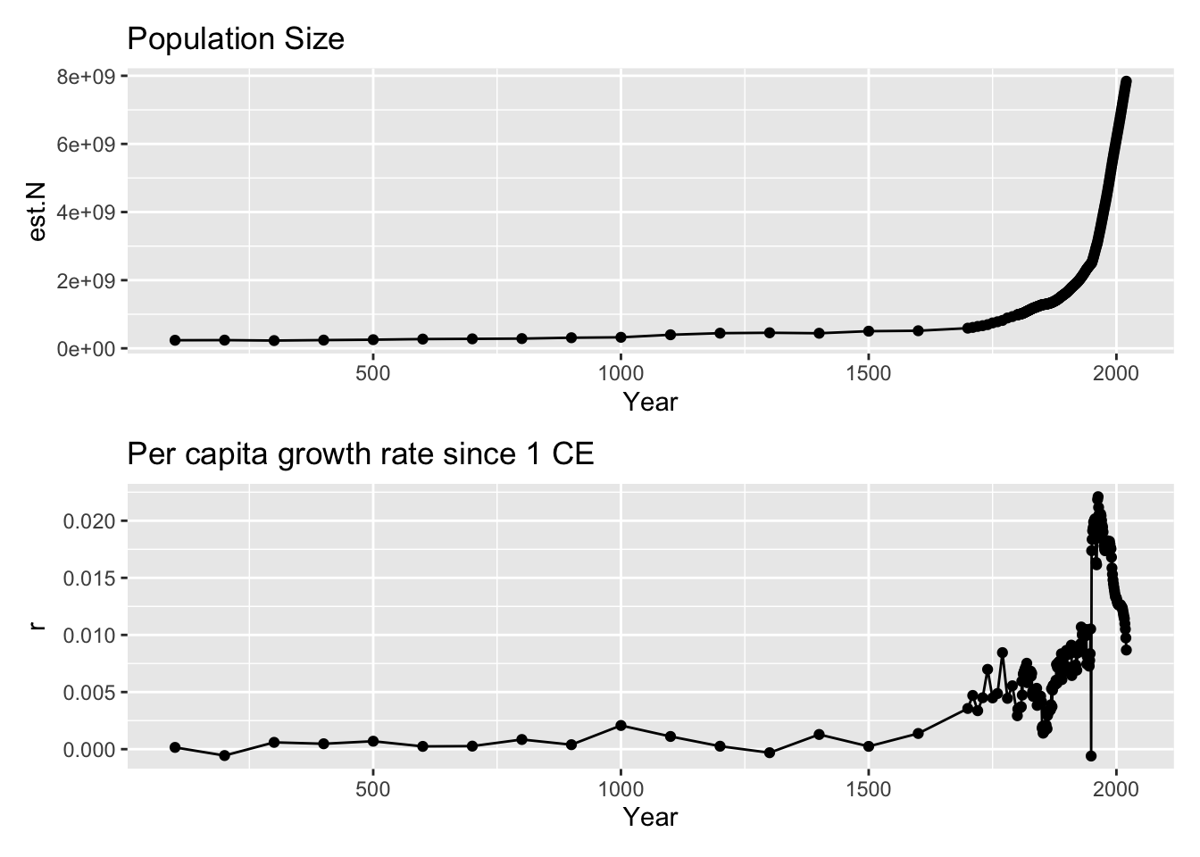
# filter in all years greater than or equal to 1
d.r.y1 <- d.r %>% filter(Year >= 1)

ggplot(data=d.r.y1, aes(x=Year, y=est.N)) + geom_line() +
  geom_point() + labs(title="Population Size")

ggplot(data=d.r.y1, aes(x=Year, y=r)) + geom_line() +
  geom_point() + labs(title="Per capita growth rate since 1 CE")

Figure 6.7: In the current era, per capita growth remains mostly positive, and then rises sharply and begin to fluctuate dramatically after 1500.

6.5.1 Your own interval

Make a graph of per capita growth rate for a time period of your own choosing. Select a time that is different than any other that we have shown here, and make it at least 10 years

6.5.2 How does per capita growth rate change with population size?

Large populations differ from small populations in a lot of ways. Large populations might make more waste products and do more damage to their own environment, and they also foster more interactions among individuals that might have positive or negative consequences.

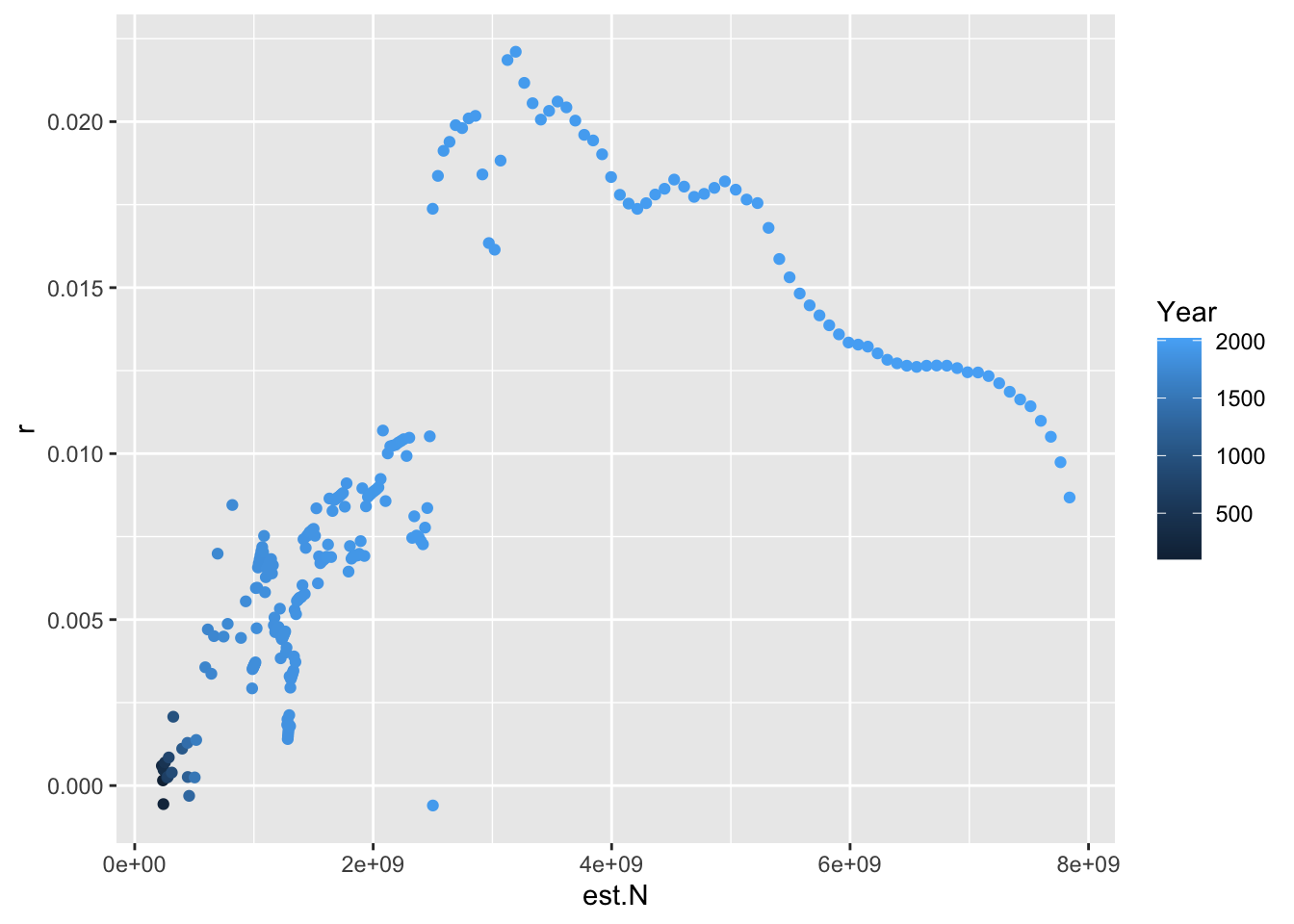
Let’s make a graph of per capita growth rate as a function of population size.

Figure 6.8: Per capita growth rate vs. population size, since 1 CE after 1500. What do you make of this? :)

6.6 Projecting into the future

Here we use our projection equation from above (\(N_t=N_0 e^{rt}\)) to make predictions about the future. Imagine a population of 100 individuals and \(r=0.02\) per year, and predict how big that population would become after thirty years. Assume that \(r\) is constant over that time period.

\[\begin{align} N_t &= N_0 e^{rt}\\ &= 100 e^{0.02 \cdot 30} = 182.21 \end{align}\]

When we take this approach, we are assuming that the population continues to grow at this rate over the projected time period. That can be a reasonable assumption over short time periods, but not over long time periods. Of course, “short” and “long” are both relative, and depend heavily of the context.

What can we learn from (Figure 6.8)? Over what time periods would it seem reasonable to assume that the human population grows at a constant rate?

6.7 Deliverables

Turn in two documents: (i) your R script, and (ii) a .docx or PDF formatted file containing the following:

Calculate by hand the exponential growth rate (r) for the years listed above in Section 6.4.2. Write out the formula, substitute the values to show you know where they belong, and then finish with the arithmetic to find \(r\).
A graph showing per capita growth rate for a time period of your own choosing, from Section 6.5.1.
If the human population continued to grow at the rate you calculated for 2020, how large would the population be in 2050? Calculate this and show your work.
What assumptions did you make in answering Question 3? Based on results for questions 1 and 2, is it likely that the human population will reach the size that you calculated for 2050? Why or why not? Use evidence in the data and the graphs above to justify your explanation.